
In order to evaluate and compare the performance of regression models, various evaluation metrics can be employed, including R2 score, MSE, RMSE, MAE, and MAPE
In the forthcoming sections, you’ll discover comprehensive explanations for each metric. Additionally, leveraging the well-known “Diabetes” dataset from the LARS paper, a practical Python example will demonstrate the step-by-step computation of each metric. You’ll also explore the utilization of scikit-learn methods. Finally, by employing two regression models, you’ll learn how to leverage these measures to determine the optimal choice
In all the following metrics formulas, we define:
- yi as the true dependent variable for the observation i
- yi as the predicted value for the observation i
- N as the number of observations in our dataset
- p as the number of independent variables in our dataset
1. Loading the dataset and fitting the model
1.1. Dataset
We will use the Diabetes data used in the “Least Angle Regression” paper: N=442 patients, p=10 predictors. One row per patient, and the last column is the response variable.
You can find the dataset (raw) in: https://www4.stat.ncsu.edu/~boos/var.select/diabetes.tab.txt
Let’s first import all the libraries will be needed for this article:
import pandas as pd
import pandas as pd
import numpy as np
from sklearn.preprocessing import StandardScaler
from sklearn.preprocessing import normalize, Normalizer
from sklearn.linear_model import LinearRegression, Lasso
from sklearn.metrics import r2_score, explained_variance_score, mean_squared_error, mean_absolute_error
from sklearn.metrics import mean_absolute_percentage_error, median_absolute_error

import matplotlib.pyplot as plt
import seaborn as sns
sns.set()
Then we load the dataset:
df = pd.read_csv("https://www4.stat.ncsu.edu/~boos/var.select/diabetes.tab.txt", sep="t")
print(df.shape)
df.head()
We will also normalize data, to have the same order of magnitude among the independent variables:
#### Scaled data: X-mean:
# Start by subtracting the mean with StandardScaler, without dividing by the std(with_std=False)
df_sc = StandardScaler(with_std=False).fit_transform(df)
df_sc = pd.DataFrame(data=df_sc, columns=df.columns)

#### Normalize data: divide each feature by its L2 norm
# If axis=0 no need to transpose, this available in "normalize" method but not in "Normalizer"
df_norm = normalize(df_sc.iloc[:,:-1],axis=0,norm='l2')
#or transpose the dataframe: (as axis=1 is the default value )
#df_norm=normalize(df_sc.iloc[:,:-1].T,norm='l2')
#(not to forget to transpose the results too, to go back to the initial shape)

df_norm = pd.DataFrame(data=df_norm, columns=df.columns[:-1])

df_norm['Y'] = df_sc['Y']
print("Normalized data: Scaled data/L2 norm")
df_norm.head()
1.2. Model to fit
To illustrate the computation of the different evaluation metrics for regression models, step by step, let’s take the predicted values given by the OLS model “y_predict_ols”. In this example we will not be splitting the dataset to train and test sets. It’s not the objective of this notebook.
features = df.columns[:-1]
X = df_norm[features]
y = df_norm['Y']

#### OLS: Ordinary Least Square
reg_ols = LinearRegression(fit_intercept=False)
reg_ols.fit(X,y)
#Predict values
y_predict_ols = reg_ols.predict(X)
2. Evaluation metrics for regression models:
2.1. R2 score
Definition
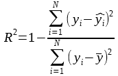
R2 score or the coefficient of determination measures how much the explanatory variables explain the variance of the dependent variable. It indicates if the fitted model is a good one, and if it could be used to predict the unseen values.
The best value of R2 is 1, meaning that the model is a perfect fit of our dataset. It could be 0, meaning that the model is a constant and it will always predict the expected average value of the dependent variable y, regardless of the input variables. It could also be negative, the model could be arbitrarily worse.
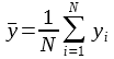
With yi the predicted value for the observation i, and y is the average value of the dependent variable:
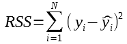
Let’s introduce another measure RSS “Residual Sum of Square” which as its name indicates, compute the square of the residual error (difference between the real and the predicted value):
We can then, write the formula of the R2 as:

By adding more and more independent variables to the dataset, the R2 score will be mechanically improved, which does not mean that those variables are really improving the accuracy of the prediction. Therefore, the adjusted R2 is introduced to provide a more precise accuracy by taking into account how many independent variables are used:

Computed
df_errors = pd.DataFrame()
df_errors['y_true'] = y
df_errors['yhat'] = y_predict_ols

df_errors['y_yhat'] = df_errors['y_true'] - df_errors['yhat']
df_errors['(y_yhat)**2'] = df_errors['y_yhat']**2

mean_y = df_errors['y_true'].mean()
df_errors['(y_ymean)**2'] = (df_errors['y_true']-mean_y)**2

r2_recomp = 1-(np.sum(df_errors['(y_yhat)**2'])/np.sum(df_errors['(y_ymean)**2']))
r2_recomp
0.5177484222203499
sklearn
r2_sk_learn = r2_score(y, y_predict_ols)
r2_sk_learn
0.5177484222203499
Both
print("r2 recomputed:",r2_recomp, ", r2_sk_learn:",r2_sk_learn)r2 recomputed: 0.5177484222203499 , r2_sk_learn: 0.5177484222203499
Let’s Visualize
plt.scatter(y_predict_ols,y)
plt.plot(y,y,'-r')
plt.annotate(r"R2={0}".format(round(r2_recomp,3)), xy=(200, 200),xytext=(-65, -10), textcoords='offset points',
             fontsize=12)
plt.xlabel("y_predict_ols")
plt.ylabel("y_true")
plt.title("Regression: Predicted vs True y")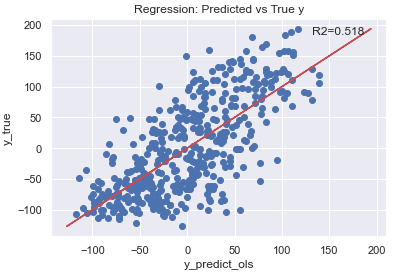
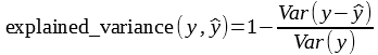
2.2. Explained Variance score
Definition
The explained variance score is computed as:
With:
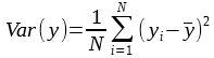
and:
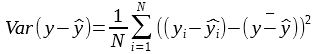
When the residuals have 0 mean, the explained variable score becomes equal to R2 score:
Computed
N=y.shape[0]

df_errors = pd.DataFrame()
df_errors['y_true'] = y
df_errors['yhat'] = y_predict_ols

mean_y = df_errors['y_true'].mean()
df_errors['(y_ymean)**2'] = (df_errors['y_true']-mean_y)**2

var_y = np.sum(df_errors['(y_ymean)**2'])/N

df_errors['y_yhat'] = df_errors['y_true']-df_errors['yhat']
mean_yyhat = df_errors['y_yhat'].mean()
df_errors['(y_yhat_yyhatmean)**2'] = (df_errors['y_yhat']-mean_yyhat)**2

var_yyhat = np.sum(df_errors['(y_yhat_yyhatmean)**2'])/N

explained_variance_recomp = 1-var_yyhat/var_y
explained_variance_recomp
0.5177484222203499
sklearn
explained_variance_sklearn = explained_variance_score(y, y_predict_ols)
explained_variance_sklearn
0.5177484222203499
Both
print("Explained variance recomputed:",explained_variance_recomp,", Explained variance from sk_learn:",
explained_variance_sklearn)
Explained variance recomputed: 0.5177484222203499 , Explained variance from sk_learn: 0.5177484222203499
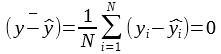
One can see that the Explained Variance and the R2 score are equal. That’s because the mean of the residual is ~0:
mean_yyhat = df_errors['y_yhat'].mean()
mean_yyhat
-4.4810811672653376e-14
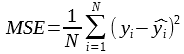
2.3. MSE: Mean Squared Error
Definition
Mean square Error compute the average squared error between the true value and the predicted one:
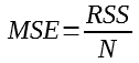
We can recall here that the RSS (Residual Sum of Square):
Then:
It gives more importance to the highest errors, thus it’s more sensitive to outliers.
Computed
N=y.shape[0]
df_errors = pd.DataFrame()
df_errors['y_true'] = y
df_errors['yhat'] = y_predict_ols
df_errors['y_yhat'] = df_errors['y_true']-df_errors['yhat']
df_errors['(y_yhat)**2'] = df_errors['y_yhat']**2

mse_recomp = np.sum(df_errors['(y_yhat)**2'])/N
mse_recomp
2859.69634758675
sklearn
mse_sklearn = mean_squared_error(y, y_predict_ols)
mse_sklearn
2859.69634758675
Both
print("MSE recomputed:",mse_recomp, ", MSE from sk_learn:",mse_sklearn)
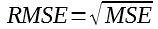
2.4. RMSE: Root Mean Squared Error
Definition
RMSE is the root squared of MSE
Computed
rmse_recomp = np.sqrt(mse_recomp)
rmse_recomp
53.47612876402657
sklearn
rmse_sklearn = mean_squared_error(y, y_predict_ols,squared=False)
rmse_sklearn
53.47612876402657
Both
print("RMSE recomputed:",rmse_recomp, ", RMSE from sk_learn:",rmse_sklearn) RMSE recomputed: 53.47612876402657 , RMSE from sk_learn: 53.47612876402657
2.5. MAE: Mean Absolute Error
Definition
MAE is the mean absolute error, is more robust to outliers than the MSE:
Computed
N = y.shape[0]

df_errors = pd.DataFrame()
df_errors['y_true'] = y
df_errors['yhat'] = y_predict_ols
df_errors['y_yhat'] = df_errors['y_true']-df_errors['yhat']
df_errors['abs(y_yhat)'] = df_errors['y_yhat'].abs()

mae_recomp = np.sum(df_errors['abs(y_yhat)'])/N
mae_recomp
43.27745202531506
sklearn
mae_sklearn = mean_absolute_error(y, y_predict_ols)
mae_sklearn
43.27745202531506
Both
print("MAE recomputed:",mae_recomp, ", MAE sklearn:",mae_sklearn)MAE recomputed: 43.27745202531506 , MAE sklearn: 43.27745202531506
2.6. MAPE: Mean Absolute Percentage Error
Definition
MAPE also known as Mean Absolute Percentage Deviation (MAPD). This measure is sensitive to relative errors. It’s also insensitive to a global scaling of the target value.
It’s also more robust to outliers than MAE.

With 𝛆 a very small strict positive value, to avoid undefined value when dividing by a value of y=0.
The score could be high when the y is small, or when the difference of the absolute value is high.
Computed
N = y.shape[0]
epsilon = 0.0001

df_errors = pd.DataFrame()
df_errors['y_true'] = y
df_errors['yhat'] = y_predict_ols
df_errors['y_yhat'] = df_errors['y_true']-df_errors['yhat']
df_errors['abs(y_yhat)'] = df_errors['y_yhat'].abs()
df_errors['abs(y_true)'] = df_errors['y_true'].apply(lambda x: max(epsilon,np.abs(x)))
df_errors['(y_yhat)/y'] = df_errors['abs(y_yhat)']/df_errors['abs(y_true)']

mape_recomp = np.sum(df_errors['(y_yhat)/y'])/N
mape_recomp
3.2636897018293114
sklearn
mape_sklearn = mean_absolute_percentage_error(y, y_predict_ols)
mape_sklearn
3.2636897018293114
Both
print("MAPE recomputed:",mape_recomp, ", MAPE sklearn:",mape_sklearn)MAPE recomputed: 3.2636897018293114 , MAPE sklearn: 3.2636897018293114
2.7. MedAE: Median Absolute Error
Definition
MedAE metric computes the median of all absolute residual values:

This metric does not take into consideration the outliers.
Computed
N = y.shape[0]
epsilon = 0.0001

df_errors = pd.DataFrame()
df_errors['y_true'] = y
df_errors['yhat'] = y_predict_ols
df_errors['y_yhat'] = df_errors['y_true']-df_errors['yhat']
df_errors['abs(y_yhat)'] = df_errors['y_yhat'].abs()

medae_recomp = np.median(df_errors['abs(y_yhat)'])
medae_recomp
38.5247645673831
sklearn
medae_sklearn = median_absolute_error(y, y_predict_ols)
medae_sklearn
38.5247645673831
Both
print("MedAE recomputed:",medae_recomp, ", MedAE sklearn:",medae_sklearn)MedAE recomputed: 38.5247645673831 , MedAE sklearn: 38.5247645673831
3. Evaluation metrics to compare among regression models
We will use 2 regression models, to fit the data and evaluate their performance. As explained at the beginning, we will not be splitting the dataset to train and test sets. It’s not the objective of this notebook.
features = df.columns[:-1]
X = df_norm[features]
y = df_norm['Y']

#### OLS: Ordinary Least Square
reg_ols = LinearRegression(fit_intercept=False)
reg_ols.fit(X,y)
#Predict values
y_predict_ols = reg_ols.predict(X)

####LASSO
reg_lasso = Lasso(alpha=1,fit_intercept=False) #Without cross-validation to find the best alpha, it's not the objective here
reg_lasso.fit(X,y)
#Predict values
y_predict_lasso = reg_lasso.predict(X)
Now that we fit the models, let’s compute the different metrics for each of them:
predicted_values = [y_predict_ols,y_predict_lasso]
models = ['OLS','LASSO']
measures_list = []
i=0


for y_predict in predicted_values:
    r2 = r2_score(y, y_predict)
    explained_variance = explained_variance_score(y, y_predict)
    mse = mean_squared_error(y, y_predict)
    rmse = mean_squared_error(y, y_predict,squared=False)
    mae = mean_absolute_error(y, y_predict)
    mape = mean_absolute_percentage_error(y, y_predict)
    medae = median_absolute_error(y, y_predict)
    measures_list.append([models[i],r2,explained_variance,mse,rmse,mae,mape,medae])
    i=+1


df_results = pd.DataFrame(data=measures_list, columns=['model','r2','explained_var','mse','rmse','mae','mape','medae'])
df_results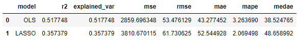
As shown in the results, the R2 is higher for the OLS (0.52) than the Lasso model (0.36) (even if the value in absolute terms is not that high). At this stage, we can assume that the OLS is a better model than the Lasso for our dataset.
Furthermore, the MSE and RMSE are lower for the OLS than the Lasso. Once again, OLS is a good fit for our dataset.
MAE and MedAE are also showing better results for OLS than Lasso.
However, MAPE is lower for the Lasso than the OLS, showing that there are some values of the true y that could be high, making the relative value of the residual lower. It could be interesting to study the outliers in the dataset, and remove them if any.
Globally, the OLS model is showing better metrics than the Lasso model. Thus, between these 2 models, OLS will be a good fit for our dataset.
Summary
In this article, you have learned:
- The most imporant evaluation metrics used to assess the performance of regression models:
- R2 Score
- Explained Variance Score
- MSE: Mean Squared Error
- RMSE : Root Mean Squared Error
- MAE: Mean Absolute Error
- MAPE: Mean Absolute Percentage Error
- MedAE: Median Absolute Error
- Their mathematical formulas
- Their computation step by step using a pratical example in Python
- Their computation using scikit-learn library
- The application of these metrics to choose between 2 models: OLS and Ridge
I hope you enjoyed reading me. Did you find this ressource useful? leave me a comment to give me your feedback👇.