
In this comprehensive article, titled “Decision Tree Structure in Python” we will dive into the practical aspects of Decision Tree for Classification using Python. Throughout this journey, you will gain insights into the following:
- Fitting, predicting, and evaluating the model using the Scikit-learn library.
- Visualizing the tree structure and interpreting its components.
- Computing essential metrics such as the Gini index for each node using Python.
Furthermore, you will gain a deeper understanding of the inner workings of decision trees, including:
- Analyzing the decision path and precisely understanding the prediction process using Python.
- Plotting decision boundaries to visualize the separation regions.
- Fine-tuning hyperparameters using GridSearchCV.
For beginners, I recommend reading up to the section on “Gini Index computation” to gain a solid foundation. Additionally, make sure to explore the section on “Hyper-parameter tuning” towards the end of the article for further insights.
Before proceeding with the current article, I suggest reading Everything You Need To Know About Decision Trees (1/2) where I provide a comprehensive explanation of the theory behind decision trees. This will provide you with a solid foundation and enhance your understanding as you delve into the present article.
In the following, we will begin by loading the dataset that will serve as the foundation for all the learning exercises in this article.
Load the dataset
Let’s use the Iris dataset to practice Decision Trees classifier.
First we load the packages we will use:
import pandas as pd
import numpy as np
from matplotlib import pyplot as plt

from sklearn.model_selection import train_test_split
from sklearn.datasets import load_iris
from sklearn.tree import DecisionTreeClassifier
from sklearn import tree

from sklearn.metrics import accuracy_score
from sklearn.datasets import load_iris
iris = load_iris()
X = iris.data
y = iris.target
print("# of observations:", X.shape[0])
print("# of features:", X.shape[1])
print("Features name:",iris.feature_names)
print("Classes to predict:",np.unique(y))
print("Target names:",iris.target_names)
# # of observations: 150
# # of features: 4
# Features name: ['sepal length (cm)', 'sepal width (cm)', 'petal length (cm)', 'petal width (cm)']
# Classes to predict: [0 1 2]
# Target names: ['setosa' 'versicolor' 'virginica']
Here is an overview of the first 5 observations:
X[:5]
# array([[5.1, 3.5, 1.4, 0.2],
#        [4.9, 3. , 1.4, 0.2],
#        [4.7, 3.2, 1.3, 0.2],
#        [4.6, 3.1, 1.5, 0.2],
#        [5. , 3.6, 1.4, 0.2]])
For each class we have the same number of observations: 50 observations each.
np.unique(y, return_counts=True)
# (array([0, 1, 2]), array([50, 50, 50], dtype=int64))
Here is a statistical description of the dataset:
pd.options.display.float_format = '{:,.2f}'.format
df.describe()
The goal is to predict, given the measures (length and width), in which class the iris will fall.
Shortly, we will implement the decision tree classifier model on our dataset and delve into the machine learning process. This involves partitioning the dataset, fitting and evaluating the model, and, importantly, visualizing the structure of the decision tree.
Decision Tree Structure In Python
Split the dataset to train and test sets
X_train, X_test, y_train, y_test = train_test_split(X, y, random_state=0) #test_size=25% defaultFit the model
We fit the model with max_leaf_nodes=3 on the train set:
clf = DecisionTreeClassifier(max_leaf_nodes=3, random_state=0)
clf.fit(X_train, y_train)
Predict
y_predict=clf.predict(X_train)Evaluate the model
Let’s compute the accuracy score for our model.
There are many other measures to take into account: Recall, Precision, F1 score…We will keep it simple here, we use only the accuracy score to evaluate our model.
The accuracy score is the ratio of the correct classified samples among the total number of observations.
On the training set:
print(clf.score(X_train,y_train))
print(accuracy_score(y_train,y_predict))
# 0.9642857142857143
# 0.9642857142857143
Both methods give the same value.
The accuracy score 96.42% is very good. In real world datasets, it could be rare to get such a good score. Here, we are using a toy dataset, in which the data are cleaned and there is no missing.
On the testing set:
y_predict=clf.predict(X_test)
print(clf.score(X_test,y_test))
print(accuracy_score(y_test,y_predict))
# 0.8947368421052632
# 0.8947368421052632
The accuracy is about 89.5% which is still very high.
In reality, the model predicts a probability for each observation, and then applies the np.argmax to get the index of the maximum value. This index will be the predicted value.
For example, for the first observation:
print("Probabilities: ",clf.predict_proba(X_test[0].reshape(1,-1)))
print("Index of the max value: ",np.argmax(clf.predict_proba(X_test[0].reshape(1,-1))))
# Probabilities:  [[0.         0.02564103 0.97435897]]
# Index of the max value:  2
In the meantime, the first value in y_predict is:
y_predict[0]
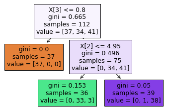
#2Visualize the decision tree structure using Python
tree.plot_tree(clf,filled=True)
plt.show()
This is the structure of the tree built by our classifier (clf with max_leaf_node=3).
There are 3 leaf nodes.
There are 2 nodes: the root node and one internal node.
In each node and leaf, there is a useful information that helps understand the splitting logic:
- It gives the best feature and threshold chosen as separator (Ex. X[3]<=0.8)
- The gini index value of the chosen feature/threshold (gini)
- Number of observations on the node (samples)
- The number of observations for each class (value)
Now that we have our decision tree structure, let’s calculate each element, in Python including the Gini index metric.
Gini Index computation
By default, the metric chosen to split the tree is the Gini index (You can modify it to use Entropy). To recall here, the lowest the value the best is the feature as a separator.
Root Node:
For the root node:
- The feature chosen is the 4th feature (petal width)
- The gini index of the training dataset before split: 0.665
- We have 112 observations in this training set.
- There are 37 observations of class 0, 34 of class 1 and 41 of class 2
Subsequently, we will compute each output for this node using Python:
Samples = 112
X_train.shape[0]
#112
value=[37, 34, 41]
df_train=pd.DataFrame(data=X_train, columns=iris.feature_names)
df_train['target']=y_train
df_train.groupby(['target'])[['sepal length (cm)']].count()
gini=0.665
The following method computes the proportion of each class in the training sets. In other terms, it computes the probability of each class (also the p2):
def compute_proprtion_class(df):
    df_proba=df.groupby(['target'])[['target']].count()/df.groupby(['target'])
                                                      ['target'].count().sum()
    df_proba.columns=['proba']
    df_proba['proba^2']=df_proba['proba']**2
    return df_proba
For training set:
df_proba=compute_proprtion_class(df_train)
df_proba
Finally the Gini index for the root node is:
gini_index= 1-df_proba['proba^2'].sum()
gini_index
#0.6647002551020409
Left of the root node
- It’s a leaf
- There are only observations (37) from class 0
- This subset is pure, so the Gini Index is 0
With Python:
Samples = 37
df_train.loc[df_train.iloc[:,3]<=0.8,:].shape[0]
# 37
value=[37, 0, 0]
Thus, this component indicates that there is only one class:
df_train.loc[df_train.iloc[:,3]<=0.8,:]['target'].unique()
# array([0])
df_train.loc[df_train.iloc[:,3]<=0.8,:].groupby(['target'])[['target']].count().rename(columns={'target':'count'})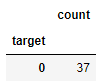
gini=0
As there is only one class (0), the probability to get this class is 1, so the gini index = 0.
Right of the root node
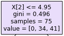
- It’s an Internal node
- There are 75 observations, from class 1 and 2
With Python:
Samples = 75
df_train.loc[df_train.iloc[:,3]>0.8,:].shape[0]
# 75
value=[0, 37, 41]
df_train.loc[df_train.iloc[:,3]>0.8,:].groupby(['target'])[['target']].count()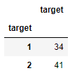
gini=0.496
df_right=df_train.loc[df_train.iloc[:,3]>0.8,:]
df_proba=compute_proprtion_class(df_right)
gini_index= 1-df_proba['proba^2'].sum()
gini_index
#0.49564444444444455
Decision Boundaries
Here is a simple visualization of the decision trees boundaries by using only two variables of our dataset:
from mlxtend.plotting import plot_decision_regions

X_train_plot = X_train[:, [0, 2]]
clf_plot = DecisionTreeClassifier(max_leaf_nodes=3, random_state=0)
clf_plot.fit(X_train_plot, y_train)
plot_decision_regions(X_train_plot, y_train, clf_plot)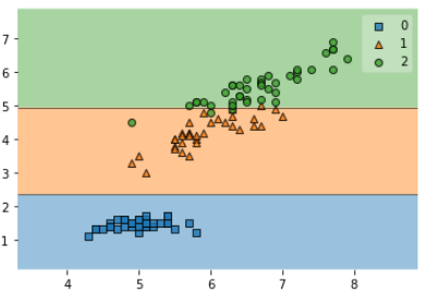
Decision Tree Structure behind the scene using Python
Presently, we will discover how to find the details of the tree structure using Python. We want to know:
- If the current node, is a node or a leaf,
- If it’s in the left or the right of the parent node,
- Which feature is the one chosen to separate the node
- The threshold values…
We can find a lot of indicators by deeply analyzing this object: clf.tree_.
In our dataset and our fitted classifier, we had this structure:
The number of nodes : 5
clf.tree_.node_count
#5
It starts with the root node, with index=0. The second node is the orange one, with index=1. It ends with the purple node, index=4.
The number of final leaves: 3
clf.tree_.n_leaves
#3
For each node: is there a left leaf?
clf.tree_.children_left
# array([ 1, -1,  3, -1, -1], dtype=int64)
Here is the explanation of the array:
- If it’s -1, meaning, no left leaf.
- If it’s different from -1, it indicates the index of the left leaf.
For example:
- The first value in the array concerns the root node. As you can see in the tree, It did have a 1 left descendante leaf. Thus, the first value of the array indicates the index of the left leaf: 1. Which is the orange leaf.
- The second value concerns the second node in the tree, which is the orange leaf. So the leaf has no left leaf, thus the value is -1.
- The third value concerns the third node (the one with X[2]<=4.95). This node has a left leaf, which has index 3. Thus this is the value you have on the array.
- etc, etc
For each node: is there a right leaf?
clf.tree_.children_right
# array([ 2, -1,  4, -1, -1], dtype=int64
- For the root node, it did have a right leaf, with the index =2. This is the first value in the array
- For the second leaf (orange), there is not right leaf, so the value is -1
- For the third node (first purple), there is a right leaf, which is the purple value with index=4.
From these two arrays, we know that the 2nd, 4th and 5th nodes are terminal leaves.
What are the features chosen for each node?
clf.tree_.feature
# array([ 3, -2, 2, -2, -2], dtype=int64)- For the first node, the feature with index equal to 3 (4th feature) is the one chosen as a separator
- For the second node, the value is -2, meaning there is no feature. It’s a terminal leaf.
- For the third node, the feature is the 3th one (idx=2)
What are the thresholds chosen for each node?
clf.tree_.threshold
# array([ 0.80000001, -2. , 4.95000005, -2. , -2.])- The first value 0.8 is the threshold applied to the feature in the index 3.
- When it’s -2, meaning the node is actually a final leaf.
The number of observations in each node
clf.tree_.n_node_samples
# array([112,  37,  75,  36,  39], dtype=int64)
The gini impurity for each node/leaf
clf.tree_.impurity
# array([0.66470026, 0.        , 0.49564444, 0.15277778, 0.04996713])
Decision path
How is the prediction made precisely?
Each observation in the test samples will go through the tree structure.
Given the sample features values, each node will decide if the sample goes left or right until it meets a final leaf. The majority class in the terminal leaf to which the sample belongs will be the predicted value.
sample_id=0
print("First sample features in the test set", X_test[sample_id].reshape(1,-1))

predict_class=clf.predict(X_test[sample_id].reshape(1,-1))[0]
print("The predict class for the sample=",sample_id," :",predict_class)

leaf_id=clf.apply(X_test[sample_id].reshape(1,-1))
print("The final leaf on which the observation falls", leaf_id)

# First sample features in the test set [[5.8 2.8 5.1 2.4]]
# The predict class for the sample= 0  : 2
# The final leaf on which the observation falls [4]
Let’s use deicion_path methods to determine the nodes through which the sample passed :
for idx, node_id in enumerate(node_index):
    is_leaf="It's not a leaf"
    idx_feature=clf.tree_.feature[node_id]
    majority_class=None

    if clf.tree_.feature[node_id]==-2:
        is_leaf="It's a leaf"
        majority_class=np.argmax(clf.tree_.value[node_id])

    if node_id in clf.tree_.children_left:
        sens_leave='Left Node'
    elif node_id in clf.tree_.children_right:
        sens_leave='Right Node'
    else:
        sens_leave='Root Node'

    to_print= majority_class

    if majority_class==None:
        print(
            "Step=",idx,"n",
            "     We are in the",sens_leave,
            ",node_id=",node_id,",",is_leaf,
            ", Best feature idx=",idx_feature,
            ", # of samples per class",clf.tree_.value[node_id],
              )
    else:
        print(
            "Step=",idx,"n",
            "     We are in the",sens_leave,
            ",node_id=",node_id,",",is_leaf,
            ", # of samples per class",clf.tree_.value[node_id],
            ", majority class= predicted value", np.argmax(clf.tree_.value[node_id])
              )

# Step= 0
#       We are in the Root Node ,node_id= 0 , It's not a leaf , Best feature idx= 3 , # of samples per class [[37. 34. 41.]]
# Step= 1
#       We are in the Right Node ,node_id= 2 , It's not a leaf , Best feature idx= 2 , # of samples per class [[ 0. 34. 41.]]
# Step= 2
#       We are in the Right Node ,node_id= 4 , It's a leaf , # of samples per class [[ 0.  1. 38.]] , majority class= predicted value 2
Let’s recall here the values of this observation:
# First sample features in the test set [[5.8 2.8 5.1 2.4]]
- At the beginning, the sample goes naturally through the root node, node_id=0.
- As the value of the fourth feature is 2.4, more than 0.8, the sample falls in the node at the right side, node_id=2.
- Then the value of the third feature is 5.1 which is more than the threshold at this node 4.95, so the feature goes to the right side again. It falls on the purple final leaf, node_id=4, on which class=2 has the majority vote. Thus the predicted value of the this observation is 2
Hyper-parameters Tuning
Hyper-parameters are not learnt by the model, they are input to the model (like ‘max_depth’, ‘max_leaf_nodes’ for Decision Trees).
We don’t know which value will give the best estimator. Thus, we need to test several values as inputs to the model and keep the one giving the best performance.
GridSearchCV
GridSearchCV helps perform this search, while cross-validating the data (using 5-fold by default).
We input a grid of parameters to GridSearchCV. It fits the model, with all the possible combinations of parameter values, to our dataset. It evaluates each combination and keeps the best one in memory.
Let’s practice:
from sklearn.model_selection import GridSearchCVLet’s test several values of max_depth, min_samples_leaf and max_leaf_nodes.
X = iris.data
y = iris.target

X_train, X_test, y_train, y_test = train_test_split(X, y, random_state=0) #(25% default)

parameters = {'max_depth':[2,3,4,5,6], 'min_samples_leaf':[10,5,1],'max_leaf_nodes':[3,4,5,7,10]}
dt = DecisionTreeClassifier()
clf = GridSearchCV(dt, parameters)
clf.fit(X_train,y_train)
We can then retrieve the best parameters and the best score:
best_params=clf.best_params_
best_params
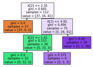
# {'max_depth': 3, 'max_leaf_nodes': 4, 'min_samples_leaf': 1}The best estimator is when max_depth=3, max_leaf_nodes=4 ,min_samples_leaf=1.
The score corresponding to these best parameters :
clf.best_score_
# 0.9644268774703558
Here is the best classifier:
clf.best_estimator_
# DecisionTreeClassifier(max_depth=3, max_leaf_nodes=4)
Fit the best estimator, Predict and Evaluate
We will fit our training by this best estimator, test and evaluate the model :
clf_best = clf.best_estimator_
clf_best.fit(X_train,y_train)
clf_best.score(X_train,y_train)
# 0.9821428571428571
The training accuracy is 98.2%. It is much higher than the first model 96.4% with max_leaf_nodes=3, and without any tuning.
The predicted values of the test set:
y_predict=clf_best.predict(X_test)
print(clf_best.score(X_test,y_test))
print(accuracy_score(y_test,y_predict))
# 0.9736842105263158
# 0.9736842105263158
Also, the test accuracy is way better than the first model: 97.37% vs 89.5%
Visualize the decision tree structure
Here is the structure of this best classifier:
Summary
In this article, you have gained knowledge on using a decision tree classifier within Python. You have learned how to perform model fitting, prediction, and evaluation. Additionally, you explored techniques to visualize the tree structure and compute various elements, such as the gini impurity metric. The article also covered plotting decision boundaries, delving into the tree structure in more detail, understanding decision paths, and tuning hyperparameters using Grid Search to find the optimal model.
If you want to understand the concepts behind the decision trees and the metrics used to split the trees, you can have a look at the following articles:
- Gini Index
- Entropy
- Information Gain
- Decision Trees Definition (½)