Welcome to this article, where we delve into the world of decision trees and explore the powerful CART (Classification and Regression Trees) algorithm. In this comprehensive guide, we provide a straightforward introduction to decision trees and a detailed explanation of the inner workings of the CART algorithm. Whether you are new to decision trees or seeking to deepen your understanding, this article serves as an excellent starting point.

Let’s begin

What are the decision trees?

Decision Trees serve as non-parametric models employed in supervised machine learning, with the objective of predicting a target value based on a given set of independent variables. One can use these versatile models for both regression tasks, where the target variable assumes continuous values, and classification objectives, where the target value belongs to a discrete set of values.

Decision trees offer the advantage of being visually interpretable, providing clear explanations and allowing for the interpretation of the algorithm’s decision-making process. This characteristic classifies them as “white box” models, in contrast to neural network algorithms, which are often regarded as “black boxes” due to their complex nature and limited interpretability.

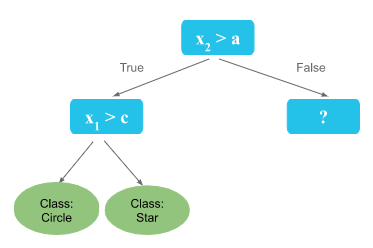
At the top of the decision tree structure, there is a root node that examines and selects a condition based on an input feature. This selection results in two branches, “True” or “False,” which lead to either a leaf node representing the final desired answer (the prediction) or to another intermediate node, also known as an internal or child node. At this intermediate node, another feature condition is examined and selected for further branching within the decision tree structure.

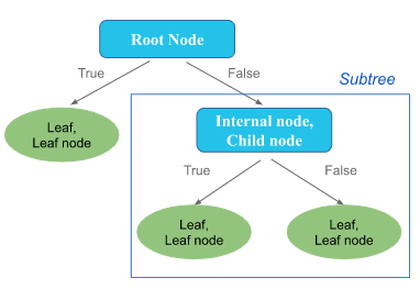
Decision Tree Structure

In the following, you will discover a comprehensive introduction to decision trees splitting and a detailed explanation of the CART algorithm, presented with clear illustrations for enhanced clarity.

Illustration of an introduction to decision trees splitting and CART algorithm

To illustrate the structure of a decision tree, let’s take the following example.

We have two features x₁, x₂, and a target value with 2 distinct classes : The circles and the stars. The goal is to build a decision tree for this dataset.

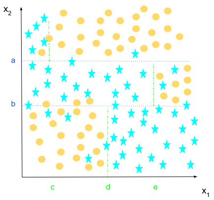
For the root node, let’s assume that x₂ > a is the best separator. 

To know how to select the best feature, I encourage you to read my articles on Entropy, Information Gain, and Gini Index.

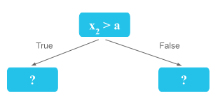
1. If x₂ > a, we will be on the left side of the tree, and end up with this subset:

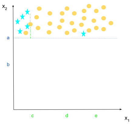
x₂>a

One can notice that we can still separate the classes according to x₁ values.

if x₁ > c, we have a majority of circle class, and if  x₁ < c we have stars.

2. If x₂ <= a, we will be on the right side of the tree, and end up with subset:

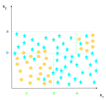
x₂<a

It’s a more heterogeneous distribution. One can use several separators. Let’s assume that x₂>b is the best separator for this node.

Let’s go to the left side of x₂ > b, and find the best separator. We have this distribution:

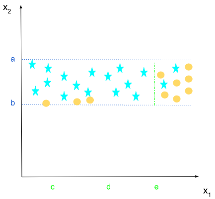
x₂<a and x₂>b

The value e of the feature x₁ seems to be the best one.

By continuing this recursive logic of splitting, the final tree will be: 

Final Decision Tree

Main ideas:

• Several linear separators are used to form non linear decision boundaries.

• Each node is an hyperplan, orthogonal to the axes. Thus easy to explain.

• The predictor is explained as a tree: each node represents the linear separator, and each leaf represents the final value to predict. it can be a class in case of classification, or a continuous value for regression.

Stopping Criteria

The splitting process concludes when a stopping criterion is satisfied. For example if we have only one observation left on the leaf, we stop the splitting nodes.

The stopping threshold for the algorithm can be reached when we achieve:

• The maximum depth of the tree

• The maximum number of leaves

• The minimum number of observations left in a node

One can define this threshold as input to the model.

Overfitting

If the minimum number of observations left in a node is 1, the risk of overfitting is high. We could then have a perfect performance of the model in the training data but a poor score in the testing data. Careful consideration must be given to selecting an appropriate threshold value to prevent overfitting.

This threshold is what we call a hyperparameter and it can be cross-validated to get the best value.

Recursive algorithms: CART Algorithm

The splitting process, we saw in the “Illustration” paragraph, is what we call recursive partitioning. The recursion is terminated when a stopping criteria is met.

The recursive process is handled by the algorithms like CART, ID3, C4.5, C5.0 and See5.

Which algorithm is implemented in scikit-learn?

In the scikit-learn library, we use CART algorithm for classification and regression. As mentioned by the scikit-learn team, CART does not handle categorical features.

Meaning, when you have a dataset in which you have one or more than independent categorical variables, you need to transform them before applying the model.

Here is how you can transform them:

Use: 
sklearn.preprocessing.OneHotEncoder
pandas.get_dummies

Do not use:
sklearn.preprocessing.LabelEncoder
This method is used to encode target values and not the features.

This method gives an ordinal data, which means there is an order between the categories. Which is wrong.

Consider a feature on which we have: Blue, Red and Green colors as values. By applying this method, you will get 0 for Blue, 1 for Red and 2 for Green. Initially there is no order between colors, but now, with this method there is one. It will lead to wrong interpretation by the model , and hence a bad prediction.

What is CART Algorithm?

CART stands for Classification And Regression Tree. Both procedures have similarities, but also some differences when it comes to the method of how to split.

In the CART algorithm, features can be continuous or categorical. The last type requires pre-processing before input into the model.

Also, the target could be either categorical or continuous.

This algorithm builds binary trees using the following steps:

• For each node (the first one being the root node), search for the best candidate among the features and the best threshold (for continuous inputs) to split the node

• The best candidate is the one for which the metric to evaluate is the best:
  • For classification: the metrics to evaluate could be Entropy, Gini Index, and Information Gain. The best candidate is the one with the lowest Entropy or Gini Index, and the highest Information Gain.
  • For Regression: the metric is a measure of the variance of the error, or simply the RSS. The lowest is the value, the better is the feature and its threshold to split the node. There are also other metrics like Friedman MSE, Poisson Deviance, Mean Absolute Error.

• After splitting the node, proceed to the child nodes and repeat the preceding steps.

• Stop the recursive process once the stopping criteria is met.

Don’t worry if you don’t know Entropy, Gini Index or Information Gain. I wrote 3 detailed articles about each one of them. 

I strongly encourage you to explore these articles, as they provide valuable insights into the underlying intuition behind these concepts and their practical application.

Pruning

Once the tree is created, the algorithm goes back through the structure and removes branches that do not add values into the prediction, and creates leaf nodes in their place.

Summary

Throughout this article, you have acquired an in-depth understanding of the theoretical foundations of decision trees. Additionally, you have gained practical knowledge on how to perform tree splits, supported by clear illustrations and a comprehensive explanation of the CART algorithm.

To further enhance your knowledge of decision trees, this time with a practical example using Python, I invite you to read my article titled:

Decision Trees — Tree Structure In-Depth Using Python (2/2).

In this article, you will actively practice various concepts using Python, including:

• Fitting a decision tree classifier, making predictions, and evaluating its performance.
• Visualizing the structure of the decision tree.
• Actively computing each element of the tree using Python, enabling a deeper understanding of its construction process (e.g., utilizing the Gini index).
• Detailed explanations of other concepts, such as hyperparameter tuning and plotting decision boundaries.

I trust that you found value in reading this article. I greatly appreciate your feedback, and I encourage you to leave a comment 👇 to contribute towards enhancing the quality of my articles.