In this article, we will explore the concept of entropy and its crucial role in decision trees. Entropy quantifies uncertainty in data and provides insights into its structure, making it an essential tool in information theory and machine learning. We will understand the intuition behind this metric, its relationship with probability, and its practical application in decision tree models. We will provide a step-by-step example to compute entropy, allowing you to grasp its practical implementation in building decision trees.

What is Entropy?

Entropy is a measure, as average, of the uncertainty of the possible outcomes of a random variable.

It’s used for classification in decision trees models. This measure helps to decide on the best feature to use to split a node in the tree. This is a very powerful and useful metric. It’s also used in Information Gain measure, which could also be used in decision trees model.

For example, the different outcomes coming from a fair coin flip (two equally outcomes) constitute less uncertainty than the ones coming from a roll of a die (six equally outcomes). The first one has a lower entropy, and the second one has a higher one.

This metric used in machine learning comes from Information Theory and was developed by Claude Shannon in 1948.

Visualization and Intuition of Entropy

We can talk about Entropy as a measure of uncertainty or impurity or surprise or information value in a group of observations. All these concepts are related. 

Here is an explanation. Let’s assume we have these 3 groups:

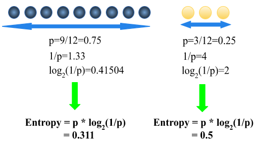
• In the first square (leftmost one), we have 6 yellow balls and 6 blue balls. So the probabilities to pick one yellow ball or 1 yellow blue are equals (6/12). In this case, we have an equal uncertainty. Both outcomes are equally likely. The entropy is equal in both cases. There is a higher disorder and lower information value.

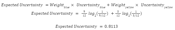
• In the second square, we have 9 blue balls and 3 yellow balls. There is more probability to pick one blue ball (9/12) than a yellow ball (3/12). 
  • In this case I’m more certain to pick a blue ball than a yellow one. 
  • For the blue balls, the certainty is higher, thus the entropy is lower. Inversely, for yellow balls, the certainty is lower, thus the measure is higher. 
  • The overall certainty of this square is higher than the first one, thus the metric value is lower. There is more information value.

• In the last square, there are only blue balls. I’m certain 100% to get a blue ball. There is no uncertainty, thus the metric value is 0.

What we need to understand from this figure is the relationship between the probability of an outcome, its uncertainty and its entropy: 

• The greater the likelihood of an outcome occurring, i.e. the more certain we are of getting that outcome, the lower is the entropy. So the entropy is inversely related to the probability.

• In other terms, the entropy is related to the uncertainty. The more uncertain we are to get an outcome, the more important is the entropy.

Mathematical formula

Intuition

As the entropy and uncertainty are inversely related to the probability, we want to write it as : Uncertainty=1/p.

Let’s go back to the last square in our figure: 

• The probability of picking one blue ball is 1. 
• We want the entropy(uncertainty) to be 0 then.

But if we only express the uncertainty as a function of 1/p, we will get Uncertainty= 1 instead of 0. To solve this issue, a log function is introduced :

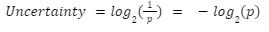
In the second square of the illustration, we have: 

For blue balls, the probability to pick one ball is 9/12, and for yellow ones is 3/12. 

So what is the expected uncertainty for this whole square to pick one blue or one yellow ball?

The global expected Uncertainty of the whole square is the weighted average uncertainty for each color: 

In other words: 

In other terms, the expected uncertainty is what we call the Entropy. It’s also the sum of 2 entropies : The blue one and the yellow one.

On one hand the uncertainty of getting one yellow ball is high, so is the entropy 0.5. On the other hand, the uncertainty to get one blue ball is low, so is the entropy 0.311.

Final Formula

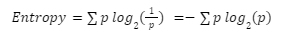
The final formula of the entropy is: 

How is the Entropy used in the Decision Trees model?

In the introduction, I explain that this metric is used as a metric in the decision trees classification model to decide which feature and value to choose to split each node in the tree.

For each node, we study every feature in the dataset by computing its entropy. The lowest is this metric, the better is the feature.

Here are the steps to follow to compute this metric and compare among the features:

• For each node:
  • Take a feature
  • Use it to split the node, on the left and right side, by creating two subsets
  • Compute the entropy of each subset/side
  • Compute the average value of the entropy for this subtree (left + right)
  • Repeat again the above steps by selecting another feature from the dataset
  • Compare all entropies computed for the different features
  • Take the lowest metric value, and thus select the corresponding feature to split the current node

• Go to the next node, and repeat the logic again, until you build the tree.

• Stop the splitting once the stop criteria of the tree is met.

Practical example

Here is an example of a dataset for which we need to build a tree, to understand how we use entropy.

          They are fake data, built just for illustration

Let’s imagine that this dataset is gathered by a bank that wants to score clients.

A client having a good credit note, will have access to a loan with the bank. And the client, having a bad note, will see his request refused by the bank.

The goal is to predict the credit note of a client, based on his/her information: savings, assets, and salary.

We want to build a tree for this dataset. The first question is what would be the best feature (Savings, Assets, Salary) to begin with in the root node?

General entropy

To do that, let’s first compute the general entropy of the dataset, before any split.

• We have 4 “Good” notes and 3 “Bad” notes.

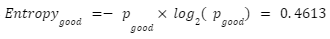
• The probability to have a “Good” note is: 

• It’s entropy is:

• The probability to have a “Bad” note is: 

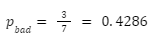
• It’s entropy is: 

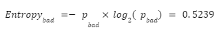
On one hand, there is more uncertainty about getting a “Bad” note, so its entropy is high. On the other hand there is less uncertainty about getting a “Good” note, so its entropy is low.

The general Entropy of this dataset is: 

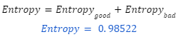
The metric value is high.

Root Node and entropy

Now, you need, for each feature in the dataset, to build a sub tree and compute the entropy.

In the following, the illustration of the calculation will be done for 1 categorical feature and 1 continuous feature:  “Savings” and “Salary”. I let you practice with the other features.

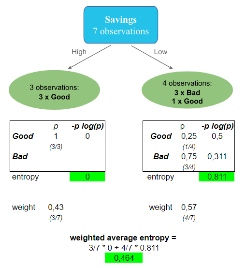
Feature 1 – Categorical: Savings

For Savings for example: 

• If “Savings” is High, we are on the left side of the subtree. There are 3 observations and they are all having Good as a credit note. So the entropy on this side of the tree is 0.

• If “Savings” is Low, we are on the right side of the subtree. There are 4 observations. 3 of them are having Bad as a credit note, and 1 observation is having Good. The entropy in this side is computed and is equal to 0.8111.

• The weighted entropy of this subtree is computed as the weighted metric value of the 2 branches. It’s equal to 0.464.

• By using “Savings as a candidate for the root node, we get 0.464 as entropy.

Feature 2 – Continuous: Salary

As the Salary feature is a continuous variable, the method to find the condition to use to split the subtree needs more computation:

• We need first, to sort the dataset based on the salary from the smallest to the largest.

• Then, we compute the average salary between two successive values. For example, the average between 20 and 25 is 22.5.

• We consider each of these values as a splitting candidate and we compute the entropy.

Let’s now take 22.5 as an example of splitting value for the root node, and compute the correspondent entropy:

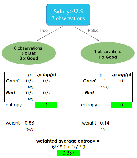
• On the left side, there are 6 observations higher than 22.5: 3 Good and 3 Bad. This is a perfect uncertainty, leading to metric value equal to 1

• On the right side, only one observation: Good. So the entropy is 1

• The overall entropy of this subtree is 0.857. This is better than the one computed for Assets, but it’s still greater than the one computed for Savings.

• Savings for the moment stays the best candidate for the root node

Now, you understand how the computation of the entropy is handled for each subtree. You can continue on your side as an exercise.

Results

Here is a summary of the different subtrees for the root node:

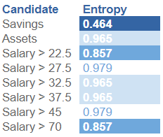
Savings has the lowest Entropy. It will be the best candidate for the split on the root node.

For the internal nodes, the same method will be applied, by taking only the observations included in this sub-tree.

Log loss

Important: in Scikit-learn log-loss is also a type of entropy. Both methods are triggering entropy computation.

Summary

The most important thing to keep in mind is that the lowest is the entropy of a subtree, the better is the feature (and the threshold value) used to split the node of this tree.

Now that you master the computation of this metric, you can have a look at another one which is the Information Gain metric.

In this article, you have learned about Entropy, used in decision trees classification:

• Its definition
• Its mathematical formula and the intuition behind
• How to use it to build a tree: Its computation, step by step, feature by feature using an example of a dataset

I hope you enjoyed reading this article.

Was the explanation clear and useful? Tell me in the comments, I appreciate your feedback 👇.