Linear Regression in Scikit-learn and StatsModel

Beginners ML, Machine Learning

In this comprehensive guide, Linear Regression in Scikit-learn and StatsModel, we will explore the powerful technique of Ordinary Least Squares (OLS) regression and its applications in predictive modeling. You will learn how to effectively utilize this method to predict values, and we will delve into the usage of both the Scikit-learn and StatsModels libraries for fitting the regression model. Furthermore, we will demystify the interpretation of p-values and other crucial results, equipping you with the necessary knowledge to extract meaningful insights from your regression analyses.

Linear Regression – Ordinary Least Squares (OLS)

Linear regression model is a function that expresses a relationship between one or more independent variables x_i (also called the features or explanatory variables) and a target variable y_i.

Simple linear regression model:

Simple Linear regression model is a regression with only one dependent variable:

With i the i-th observation in the dataset, and ɛ_i the error term.

The parameters of the model are w0, the intercept, and w1 the slope. We call these parameters the regression coefficients (or beta).

Multiple linear regression model:

Multiple Linear regression model is regression with several dependent variables:

With k is the number of the explanatory variables, and i is the i-th observation.

Representation and Cost function

Let’s focus on a simple linear regression model, to be able to explain and represent simply the different concepts that will be used to estimate the parameters of the model.

Let’s assume we have one independent variable X and we want to predict y:

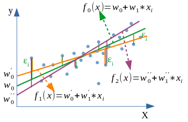
The function of the green line is our regression model:

The parameters of this model, the intercept w₀and the slope w₁ will be used to predict y_i , with an error term ɛ_i.

This error term is the difference between the predicted value of y_i and its projection on the regression line. It’s also called the residual.

The goal of the regression model is to minimize this error term, to find the line that will fit the best our dataset. In other term, the objective is to find the best estimate of w0 and w1 that will minimize the error term ɛ_i.

To be able to determine which line is the best fit for our dataset f₀, f₁ or f₂ as shown in the following figure, we need first to introduce a quality metric: RSS (Residual sum of squares)

RSS: Residual sum of squares

RSS is the sum of the squared difference between the predicted value, using the parameters w₀ and w₁ (yi=w0+w1xi), and the real one y. Otherwise, RSS is the sum of squared error term ɛ_i:

In other terms, RSS could be written with w₀ and w₁:

The RSS is our cost function, the smallest is the value, the smallest is the distance between our predicted value and our real one, and the best is the regression line.

Now we will discuss the algorithm that will minimize this cost over all possible values of w₀ and w₁:

(You can download for free the sample ebook of linear regression to have more information about the algorithm used – Gradient Descent to minimize the cost function).

All this logic is developed in Scikit-learn and StatsModels library.

Before practicing with Python, let’s have a look at the global process to follow when you’re working with machine learning models.

Process of Fitting the models in machine learning

Prior to delving into the practical Python example of applying Linear Regression using Scikit-learn and StatsModels, it is essential to familiarize yourself with the necessary steps to utilize machine learning models effectively. These steps include:

Import libraries you need to work with in you project
Load your dataset
Split the dataset to train, and test sets : The goal is to train your model on the training sets, and compute the accuracy of the model on the test sets, which was not discovered yet by the model (to be the most realistic)
Normalize your data train, and then infer this transformation to the test sets.
Fit the model
Predict
Evaluate the model

in “fit” and “predict” steps, you can use several models, and evaluate them, to keep the most performing one.

Let’s now take an example to practice.

Python: Practical example – Linear Regression (OLS) in Scikit-learn and StatsModel

Dataset overview

The dataset that we will be using in this chapter and the following ones is the “diabetes” data that has been used in the “Least Angle Regression” paper.

In this dataset we have 442 observations (patients) and 10 variables (n=442 patients, p=10 predictors). One row per patient and the last column is the response variable.

Ten baseline variables, age, sex, body mass index, average blood pressure, and six blood serum measurements, were obtained for each of n = 442 diabetes patients, as well as the response of interest, a quantitative measure of disease progression one year after baseline.

Import the libraries

Let’s import the different packages we need:

import pandas as pd
import numpy as np
from sklearn.preprocessing import StandardScaler
from sklearn.preprocessing import normalize, Normalizer
from sklearn.linear_model import LinearRegression, Lasso
from sklearn.metrics import r2_score, explained_variance_score, mean_squared_error, mean_absolute_error
from sklearn.metrics import mean_absolute_percentage_error, median_absolute_error
import matplotlib.pyplot as plt
import seaborn as sns
sns.set()

Load the dataset

df=pd.read_csv("https://www4.stat.ncsu.edu/~boos/var.select/diabetes.tab.txt", sep="t")
print(df.shape)
df.head()
#(442, 11)
sns.set()

Our features are Age, Sex, BP, S1, S2, S3, S4, S5 and S6, and the target variable is Y.

Statistical description

To have an overview of the data used:

pd.options.display.float_format = '{:,.1f}'.format
df.describe()
sns.set()

In the whole data set we have 442 observations. The maximum value of Y is 346 and the median is 140.5. The quantile 25 for Age is 38.2 and the quantile 75 is 59.

Split to train and test

Let’s split the dataset to train and test sets : (20% on test, and 80% on train):

X_train,X_test,y_train,y_test=train_test_split(df.iloc[:,:-1],df['Y'],test_size=0.2,random_state=42)
print("Train shape",X_train.shape, "Test shape", X_test.shape)
sc_x=StandardScaler()
X_train_sc=sc_x.fit_transform(X_train)
# Apply the scaling to test data sets
X_test_sc=sc_x.transform(X_test)
#Train shape (353, 10) Test shape (89, 10)

Fit the model : OLS in Scikit-Learn

Let’s fit the Ordinary Least Square model from Scikit-learn

reg_ols=LinearRegression()
#fit_intercept=True,positive=True
reg_ols.fit(X_train_sc,y_train)

Default parameters will apply, like fit_intercept=True. If you want to mody the value, you can by passing: fit_intercept=False.

We fit the OLS to the scaled train data.

The intercept and the coefficients of the fitted model are:

intercept=reg_ols.intercept_
coef_ols=[round(coef,2) for coef in reg_ols.coef_]
print("Intercept", round(intercept,2))
print( "Coefs", coef_ols)
#Intercept 153.74
#Coefs [1.75, -11.51, 25.61, 16.83, -44.45, 24.64, 7.68, 13.14, 35.16, 2.35]

Interpret the results

The intercept means that If all coefficients are 0, the value of y will be 153.74

For the slopes, for Age the coefficient is 1.75. It means if we hold all the other variables constant, when age increases by (a normalized value of) 1 year, the progression of diabetes is about 1.75 points.

Predict

#Predict values
y_train_predict=reg_ols.predict(X_train_sc)
y_test_predict=reg_ols.predict(X_test_sc)

Evaluate

Now let’s evaluate this model. We will use the R2 score.

There are many metrics to use to evaluate the model. You find in this article, a detailed list of all these metrics, including R2 score, their mathematical formula, and how they are calculated using either hand made computation in Python or scikit-learn library.

# The coefficient of determination: 1 is perfect prediction
r2_train=r2_score(y_train, y_train_predict)
r2_test=r2_score(y_test, y_test_predict)

print("TRAIN-model direct score R2: %.5f"%reg_ols.score(X_train_sc,y_train))
print("TRAIN-recomputed         R2: %.5f" % r2_train)
print("TEST                     R2: %.3f" % r2_test)

#TRAIN-model direct score R2: 0.52792
#TRAIN-recomputed         R2: 0.52792
#TEST                     R2: 0.453

R2 score for the train is about 0.528, and the test is 0.453.

Visualization

plt.scatter(y_train_predict,y_train,label='train')
plt.scatter(y_test_predict,y_test,label='test')
plt.plot(y_train,y_train,'-r')
plt.annotate(r"R2_train={0}, R2_test={1}".format(round(r2_train,3),round(r2_test,3)), xy=(180, 20),xytext=(0, 0), textcoords='offset points',
            fontsize=12)
plt.xlabel("y_predict_ols")
plt.ylabel("y_true")
plt.title("Regression: Predicted vs True y")
plt.legend()

Now let’s use StatsModels OLS.

Fit the model: OLS in StatsModels:

X_train_sc_cst=sm.add_constant(X_train_sc)
sm_ols=sm.OLS(y_train,X_train_sc_cst).fit()
print("TRAIN: R2: %.5f"%sm_ols.rsquared)
sm_ols.summary()
#TRAIN: R2: 0.52792

Interpret the results

The summary of OLS in StatsModels gives detailed statistical values of the model.

The most important values are:

R-squared
Coefficient of the intercept (const in the table)
Coefficients of the independent variables from x1 to x10, corresponding to AGE to S6: 1.75 to 2.3514.
The p-value for the intercept and for each feature.

We get the same values of coefficients as the model used in scikit-learn.

#Intercept 153.74
#Coefs [1.75, -11.51, 25.61, 16.83, -44.45, 24.64, 7.68, 13.14, 35.16, 2.35]

Predict

X_test_sc_cst=sm.add_constant(X_test_sc)
y_test_pred=sm_ols.predict(X_test_sc_cst)

Evaluate

r2_test=r2_score(y_test, y_test_pred)
print("TEST R2: %.3f" % r2_test)
#TEST R2: 0.453

Either R2 score coming from training dataset or test dataset is the same in Scikit-learn and in StatsModel.

Visualization

y_train_predict=sm_ols.predict(X_train_sc_cst)

plt.scatter(y_train_predict,y_train,label='train')
plt.scatter(y_test_pred,y_test,label='test')
plt.plot(y_train,y_train,'-r')
plt.annotate(r"R2_train={0}, R2_test={1}".format(round(r2_train,3),round(r2_test,3)), xy=(180, 20),xytext=(0, 0), textcoords='offset points',
            fontsize=12)
plt.xlabel("y_predict_ols")
plt.ylabel("y_true")
plt.title("Regression: Predicted vs True y")
plt.legend()

How do we interpret the p-values in regression?

The p-value leads to the decision to reject or not the null hypothesis.

The null hypothesis states that the coefficient is not statistically different from 0.

In other terms, if the p-value is less than a certain threshold (commonly used value is 0.05), then we reject the null hypothesis, meaning that the coefficient has an explanatory effect on the target value.

In our example: AGE, S6, S3,S4,S2 are all having a p-value greater than 0.05.

For example, for AGE the p-value is 0.583, and for S6 is 0.508.

Those features are not having an important effect on explaining the target variable.

What’s next?

What you could do next, is:

To remove the feature (in train and test sets) having the most important p-value in your model (in our case AGE).
Then refit the model.
Check again the results of the p-values, R2 score for train AND test sets.
Repeat again until you find all p-values less than 0.05, and compare the R2 scores.

If you do this exercise you will see that the R2 score for the test sets will improve: 0.463.

There are other models that better perform this logic by removing features that are not useful for the prediction: Regularization models (Sample of Linear Regression).

Summary

Throughout this article, you have gained the knowledge and expertise required to utilize Linear Regression in two renowned libraries, namely Scikit-learn and StatsModels. You understand now: