What is KAMA algorithm?

KAMA is a trend following indicator that aims to take into account the volatility of an asset’s price. Kama tends to follow closely the asset’s price movements. 

KAMA, used with longer periods moving average, can be used to confirm existing trends. When used within a shorter period, it can identify trading signals.

KAMA s calculated as a moving average of the volatility by taking into account 3 different timeframes (see FORMULA).

When the price crosses above the KAMA indicator, a buy signal can be triggered. When it crosses below, a sell signal can be triggered. However, as KAMA (for a shorter period) is closely following the price, one can see lots of signals generated. 

To reduce the frequency of these signals, one can apply filters, before activating any signal, like: 

• Waiting some period of time or 
• Setting a threshold percentage of the price from KAMA or
• Exploiting a longer KAMA period to assess if there is an uptrend or a downtrend. Then, comparing the short KAMA to the price (cf backtesting strategy below)

FORMULA

1- Efficiency Ratio

Change = Abs(price – price(from 10-period))    
Volatility = 10-period Rolling Sum (price – Previous price)    
ER = Change / Volatility

2- Smoothing Constant

sc_fatest = 2/(2 + 1)   
sc_slowest = 2/(30 + 1)    
SC = (ER x (sc_fatest – sc_slowest) + sc_slowest ) ^ 2

3- KAMA

First value : close mean value over 10-period    
Following values:    
Current KAMA = Previous KAMA + SC x (price – Previous KAMA)

As you can see, in the formula, I exposed KAMA(10, 2, 30) which is the one recommended by Kaufman himself. However, one can act on the different time frames, but : 

• KAMA(10, 2, 30) is the one used in the market
• You can modify 2 per another timeframe, to calculate smoothed version of KAMA to confirm the existing trend before using the shorter one to generate signals (see implementation part)

How to implement KAMA in Python from scratch?

Load a dataset: Amazon stock prices

import pandas as pd
import numpy as np
import datetime as dt

import matplotlib.pyplot as plt
import seaborn as sns
sns.set()

from pandas_datareader import data as pdr
import yfinance as yfin

yfin.pdr_override()

datetime_end=dt.datetime.today().date()
df = pdr.get_data_yahoo('AMZN', start='2022-01-01', end=datetime_end)

df.head()

Here is the method to use:

def kama_indicator(price, period=10, period_fast=2, period_slow=30):
   
    #Efficiency Ratio
    change = abs(price-price.shift(period))
    volatility = (abs(price-price.shift())).rolling(period).sum()
    er = change/volatility
   
    #Smoothing Constant
    sc_fatest = 2/(period_fast + 1)
    sc_slowest = 2/(period_slow + 1)
    sc= (er * (sc_fatest - sc_slowest) + sc_slowest)**2
   
    #KAMA
    kama=np.zeros_like(close)
    kama[period-1] = close[period-1]

    for i in range(period, len(df)):
        kama[i] = kama[i-1] + sc[i] * (close[i] - kama[i-1])

    kama[kama==0]=np.nan
   
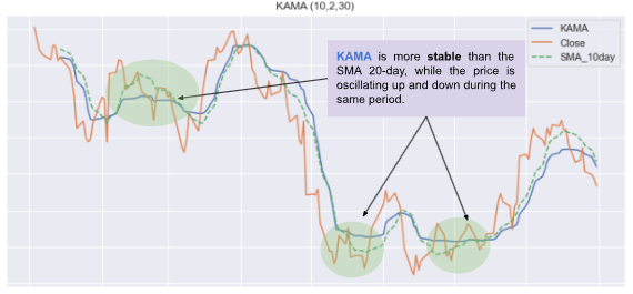
    return kama

Now, we calculate KAMA(10, 2, 30). A plot will be shown comparing KAMA to SMA (Simple moving average) 10 days:

period = 10
period_fast = 2
period_slow = 30

close=df['Adj Close']

kama2=kama_indicator(close, period, period_fast, period_slow)

df['kama2']=kama2
df['sma_10days']=close.rolling(period).mean()

figsize=(12,6)
df[['kama2','Adj Close']].plot(figsize=figsize)
df['sma_10days'].plot(linestyle="--")
plt.legend(['KAMA','Close','SMA_10day'])
plt.title("KAMA ({0},{1},{2})".format(period, period_fast, period_slow))
plt.show()

KAMA is more stable than SMA 10-days, it follows less the price movement when there is a high volatility. (see interpretation part)

Interpertation

Let’s focus on a smaller period:

df_plot=df[df.index<'2022-09-01']

figsize=(12,6)
df_plot[['kama2','Adj Close']].plot(figsize=figsize)
df_plot['sma_10days'].plot(linestyle="--")

plt.legend(['KAMA','Close','SMA_10day'])
plt.title("KAMA ({0},{1},{2})".format(period, period_fast, period_slow))                                                                                                 
plt.show()

As shown in the graph, KAMA is less sensitive to the price movement compared to the SMA 10-day. When the price movements are small, KAMA tends to follow the price closely. When the movements are wide and the noise is important, KAMA tends to follow the price from a distance, which makes it more stable (As shown in the following figure).

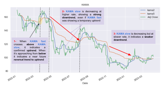
Now let’s implement KAMA(10,5, 30), which represents the slowest version of KAMA:

kama5=kama_indicator(close, period, 5, period_slow)
df['kama5']=kama5

df[['kama2','kama5', 'Adj Close']].plot(figsize=figsize)
plt.title("KAMA")
plt.show()

When KAMA fast (kama2) is approaching from below KAMA slow (kama5) (same logic applied to other moving average indicators), it indicates an approaching reversal trend. When KAMA fast crosses above KAMA slow, it confirms the uptrend (which has already started), as shown in point 1- in the graph.

When KAMA “slow” is decreasing (increasing) at a higher rate, it shows a strong downtrend (Point 2- in the graph). When the decrease is slow, it indicates a weak downtrend (Point 3- in the graph).

Backtesting our strategy

Let’s put in place a buy/sell signal based on the following indication:

• If KAMA slow is decreasing and the price fall below KAMA fast, then a sell signal is triggered
• If KAMA slow is increasing and the price crosses above KAMA fast, then a buy signal is triggered

#*********************************SIGNAL********************************
# Calculate KAMA Slow Rate Of Change (ROC)
kama_roc = df['kama5'].pct_change()

# Calculate the signal
df['signal']=np.where((kama_roc>0) & (close >= kama2),1,np.where((kama_roc<0) & (close <= kama2),-1,0))

#*********************************RETURN********************************
df['signal_shifted']=df['signal'].shift()

# Calculate the returns on the days we trigger a signal
df['returns'] = df['Adj Close'].pct_change()

# Calculate the strategy returns
df['strategy_returns'] = df['signal_shifted'] * df['returns']

# Calculate the cumulative returns
df1=df.dropna()
df1['cumulative_returns'] = (1 + df1['strategy_returns']).cumprod()


df_concat = pd.concat((df[['Adj Close','kama2','kama5','signal']],df1[['cumulative_returns']]),axis=1)

#*********************************PLOT**********************************
figsize=(12,14)
fig, (ax0,ax1, ax2) = plt.subplots(nrows=3, sharex=True, subplot_kw=dict(frameon=True),figsize=figsize)

df_concat[['Adj Close','kama2','kama5']].plot(ax=ax0)
ax0.set_title("KAMA")

df_concat[['signal']].plot(ax=ax1,style='-.',alpha=0.4)
ax1.legend()
ax1.set_title("KAMA - Signals")

df_concat[['cumulative_returns']].plot(ax=ax2)
ax1.legend()
ax1.set_title("cumulative_returns")

plt.show()

The overall return is positive:

df1['cumulative_returns'].iloc[-1]

1.005391424241043

Comparison with TA-Lib implementation

In TA-Lib, we will call the function talib.KAMA. Here is the definition:

As you can see, only one period is available in the function. This time period corresponds to the first time period we used before (=10). Therefore, in TA-Lib you cannot modify the other timeframes (2 and 30).

import talib
close=df['Adj Close']

kama_talib=talib.KAMA(close, timeperiod = 10)
df['kama_talib']=kama_talib

Let’s compare our implementation to TA-Lib one:

figsize=(8,5)
df[['kama_talib','kama2', 'Adj Close']].plot(figsize=figsize)
plt.show()

We have the exact values:

df[['kama_talib','kama2']].head(20).tail()

However in TA library, you have access to the different timeframes in the function parameter (ta.momentm.KAMAIndicator)

Summary

In this article, you have learned : 

• KAMA indicator
• How to implement it using Python from scratch
• Its interpretation
• A strategy and backest example
• TA-Lib implementation