In this article, you will discover what is TA-Lib and How to implement 2 technical Indicators in Python. You will learn:

• TA-Lib and how to install it and use it
• 2 technical indicators: Definition, Formula
• Implement them in Python from scratch
• Compare results between TA-Lib and Python implementation
• Understand the intuition behind

TA-Lib

What is TA-Lib?

TA-Lib is an open-source technical analysis library used by traders, investors and analysts to perform complex calculations on financial data and build trading strategies.

The library is written in C language and provides more than 150 technical indicators and trading functions. These indicators are used to identify trends, measure momentum, and assess the overall strength and direction of a market. 

🗨️ It can be easily integrated into various programming languages such as Python, R, and Java, making it accessible to a wide range of users. 

How To Install TA-Lib?

Detailed information is given in the README.md file, but here is how to install in Python: 

You can install from PyPI:

$ python3 -m pip install TA-Lib

Or checkout the sources and run setup.py yourself:

$ python setup.py install

It also appears possible to install via Conda Forge:

$ conda install -c conda-forge ta-lib

What are the different indicators implemented in TA-Lib?

There are different categories of indicators implemented in TA-Lib. Here is a short list: 

• Overlap Studies ( ex: Bollinger Bands)
• Momentum Indicators (Ex: ROC- Rate of Change)
• Volume Indicators (Ex: OBV – On Balance Volume)
• Volatility Indicators (Ex: ATR – Average True Range)

You can find here the exhaustive list of the indicators: https://github.com/TA-Lib/ta-lib-python/blob/master/docs/funcs.md

🗨️ The source code of the functions is written in C and it is not easy to understand. That’s why a step by step guide, explaining the formulas and implementing from scratch the indicators in Python, is needed. Have a look at my new ebook Technical Indicators using Python and TA-Lib in which I explain in-depth more than 25 technical indicators.

Now, let’s learn how to use TA-Lib and how to implement 2 technical indicators using Python from scratch? 

Loading Dataset

Let’s start by loading a dataset, and the libraries we need, for Google since Januray 2022:

import talib
import numpy as np
import pandas as pd

import matplotlib.pyplot as plt
import seaborn as sns
sns.set()

from pandas_datareader import data as pdr
import yfinance as yfin

yfin.pdr_override()

df = pdr.get_data_yahoo('GOOG', start='2022-01-01', end='2022-12-23')

df.head()

ATR: Average True Range

Average True Range is a technical indicator that measures the volatility of an asset. It’s calculated by taking the maximum of these three measures, involving the High, Low and previous Close, and then applying an exponential weighted average (EWA) with a n-period, typically 14-day.

The calculation involves two steps as described below:

FORMULA

1- Calculate the True Range (TR) value: which is the maximum value of the following:
        True 1: High – Low
        True 2: Absolute value of High – previous close
        True 3: Absolute value of Low – previous close
    TR = max(high – low, abs(high – previous close), abs(low – previous close))
   
2- Smooth the TR values using a 14-period EWA (Exponential Weighted Average):
        First value of ATR = The average of TR over 14-day period
        The following value:
    Current ATR = Current TR * 1/period + Previous ATR * (1-1/period)

One can see that the formula is directly linked to the price level of the asset, making it impossible to compare among assets.

TA-Lib: talib.ATR

period = 14
high = df['High'].values
low = df['Low'].values
close = df['Adj Close'].values
atr_talib = talib.ATR(high, low, close, timeperiod=period)
atr_talib[:20]

array([       nan,        nan,        nan,        nan,        nan,
              nan,        nan,        nan,        nan,        nan,
              nan,        nan,        nan,        nan, 4.11370629,
      4.10515555, 4.2456443 , 4.20416599, 4.23786806, 4.19012777])

How to implement Average True Return (ATR) using Python to get the same result as TA-Lib? 

period = 14
high = df['High'].values
low = df['Low'].values
close = df['Adj Close'].values
previous_close=df['Adj Close'].shift().values

tr1=high-low
tr2=np.abs(high-previous_close)
tr3=np.abs(low-previous_close)
true_range=np.max((tr1,tr2,tr3),axis=0)
true_range[0]=tr1[0]

# Average True Range 14 days period EWA:
atr=np.zeros_like(high)
atr[period]=np.mean(true_range[1:period+1])

for i in range(period+1,df.shape[0]):
    atr[i]=true_range[i]*1/period+atr[i-1]*(1-1/period)
display(atr[:20])

array([0.        , 0.        , 0.        , 0.        , 0.        ,
      0.        , 0.        , 0.        , 0.        , 0.        ,
      0.        , 0.        , 0.        , 0.        , 4.11370629,
      4.10515555, 4.2456443 , 4.20416599, 4.23786806, 4.19012777])

We get the same results as the TA-Lib function.

Contrary to what is explained in the literature,  where the first value of true range is initialized by the difference between High and Low, in TA-Lib the first value must be equal to 0. The true_range in my calculation is also equivalent to this TA-Lib function: talib.TRANGE (high, low, close), with the first value equal to nan.

Interpretation

This indicator is used only as a measure of volatility, it is not used to identify price direction. It’s used in other indicators like ADX, as said before, which can give more insights on an asset’s trend.

Let’s plot the different calculations to understand this indicator:

df["atr_talib"]=atr_talib
df['tr1']=tr1
df['tr2']=tr2
df['tr3']=tr3

figsize=(12,10)
fig, (ax0,ax1,ax2) = plt.subplots(nrows=3, sharex=True, subplot_kw=dict(frameon=True),figsize=figsize)

df['Adj Close'].shift().plot(ax=ax0,label="prev Close")
df[['High','Low']].plot(ax=ax0,style='--')
ax0.fill_between(df.index,df['High'], df['Low'], alpha=0.2)
ax0.legend()

df[['tr1','tr2','tr3']].plot(ax=ax1,style='--')
ax0.legend()

df[['atr_talib']].plot(ax=ax2)

plt.title("ATR Indicator")
plt.legend()
plt.show()

🖋️ A big volatility is recorded in early February 2022. This is due to the big difference noticed between the High and the previous close (tr2) (orange color in the second graph). The same thing can be noticed several moments during this period, like in May 2022 where this time is due to tr1 (High-Low) difference.

BBands: Bollinger Bands

Bollinger Bands is a technical indicator that measures the volatility bands of an asset’s price. There are 3 bands, the upper band, the middle band, and the lower band. The middle band is a simple moving average of the price over a period, typically 20-days. The upper (lower) band is simply 2 standard deviations above (below)  the middle band.

When the volatility of an instrument increases, the upper and lower bands widen, and when the volatility decreases, the bands shrink.

The bollinger bands could be used to identify the strength of the trend, or to determine if the asset is overbought or oversold. Based on this, it can trigger buy and sell signals.

FORMULA

1- Middle_band = Simple Moving Average (SMA) n-period. Typically 20-day
2- Upper_band = Middle_band + n_std * price standard deviation over n-period
3- Lower_band = Middle_band – n_std * price standard deviation over n-period  

   n_std is the number of standard deviation

TA-Lib: talib.BBands

The number of standard deviation above and below the middle band 

close = df['Adj Close']
upperband, middleband, lowerband = talib.BBANDS(close, timeperiod=20, nbdevup=2, nbdevdn=2)

Python Implementation: How to implement Bollinger Bands using Python to get the same result as TA-Lib?

period = 20
n_std = 2

close = df['Adj Close']

# Calculate the rolling mean and standard deviation of the close
rolling_mean = close.rolling(period).mean()
rolling_std = close.rolling(period).std(ddof=0)
# ddof=0 ==> In order to devide by N instead of N-1, to get the same results than TA-Lib

# Calculate the z-score (number of standard deviations away from the rolling mean)
zscore = (close - rolling_mean) / rolling_std

upper_band = rolling_mean + n_std * rolling_std
lower_band = rolling_mean - n_std * rolling_std

To get the same results as TA-Lib, ddof=0 must be set in the rolling standard deviation build-in function in pandas. Because the default version in pandas uses N-1 as denominator, instead of N in TA-Lib. Just to remember here the standard deviation formula:

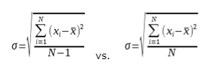
You can check by yourself the results of : talib.STDDEV vs rolling(period).std(ddof=0).

Comparing the results

Let’s compare for upper band the results of own python implementation and the one in TA-Lib:

df['upper_band_calc']=upper_band
df['upper_band_talib']=upperband   df[['upper_band_talib','upper_band_calc','middleband','rolling_mean','rolling_std','2*rolling_std']].head(25)
df[['upper_band_talib','upper_band_calc']].head(100).tail()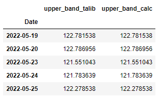

Interpretation

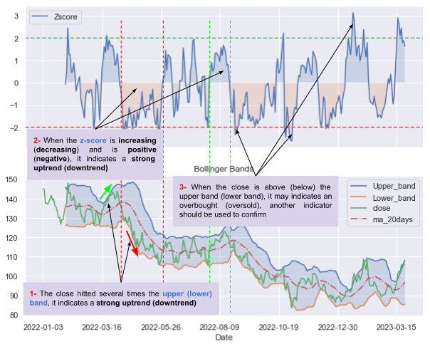
Let’s plot the close, the SMA 20-day of the price, the upper and the lower band against the z-score:

figsize=(10,8)
fig, (ax0,ax1) = plt.subplots(nrows=2, sharex=True, subplot_kw=dict(frameon=True),figsize=figsize)

zscore.plot(ax=ax0,label='Zscore')
ax0.axhline(y=2,linestyle = '--',c='g')
ax0.axhline(y=-2,linestyle = '--',c='r')
ax0.fill_between(df.index,zscore, 0, where=zscore>=0,alpha=0.2)
ax0.fill_between(df.index,zscore, 0, where=zscore<0,alpha=0.2)
ax0.legend()

upper_band.plot(ax=ax1,label='Upper_band')
lower_band.plot(ax=ax1,label='Lower_band')
close.plot(ax=ax1,label='close')
rolling_mean.plot(ax=ax1,label = 'ma_20days', linestyle = '-.')
ax1.fill_between(df.index,lower_band, upper_band, alpha=0.2)
ax1.legend()

plt.title('Bollinger Bands')
plt.legend()
plt.show()

🎯 In the graph, in point 1-, the close hitted several times the upper (lower) band, this indicates a strong uptrend (downtrend), and it also may indicate a near future mean reversion. 

🎯 When the z-score is positive and increasing, meaning the close crosses above the SMA 20-day and it’s increasing, it also identifies a strong uptrend. The same on the opposite side, when the z-score is negative and decreasing, it identifies a strong downtrend (point 2-).

🎯 When the close crosses above (below) the upper (lower) band, it means that the close deviates more than 2 standard deviations from its mean.  It may indicate (not all the time) an overbought (oversold) (point 3-). Another indicator (like CCI, RSI) can be added to confirm these signals.

Summary

In this article, you have discovered the TA-Lib library. An open-source technical analysis, providing more than 150 functions and technical indicators, widely used among traders, investors and analysts.

You also have learned how to install it, and use it. 

You have learned 2 technical indicators ATR (Average True Return) and BBands (Bollinger Bands):

• Their definition
• Their formulas
• How to implement them using TA-Lib
• How to implement them using Python from scratch
• Compare both results: some tricks explained to get the same results
• Their interpretation

I hope you enjoyed reading my article. Leave me a comment and tell if you already used Ta-Lib and for which technical indicator?