
Within this article, your understanding will be enriched regarding the Mean Reversion Trading Strategy Using Python. You will delve into its implementation, exploring three distinct approaches:
- Basic implementation
- Z-score implementation
- Statistical arbitrage implementation
Furthermore, the article will guide you through the process of backtesting each strategy, ensuring a comprehensive learning experience.
Disclaimer: The information provided in this article is for educational purposes only and should not be considered as professional investment advice. It is important to conduct your own research and exercise caution when making investment decisions. Investing involves risk, and any investment decision you make is solely your own responsibility.
What is Mean Reversion Trading Algorithm?
Mean Reversion is an algorithm that states that prices tend to revert to their long term average value. When stock price diverges from its historical average value, it means that the asset is overbought or oversold. Then, trading signals could be triggered to short or buy the instrument with the expectation that its price will revert to the mean.
In the following, you will find different implementations of the Mean Reversion Trading Strategy Using Python. But, first let’s load the dataset.
Loading Dataset
In the first and second implementation, we will use Netflix historical prices:
def download_stock_data(ticker,timestamp_start,timestamp_end):
    url=f"https://query1.finance.yahoo.com/v7/finance/download/{ticker}?period1={timestamp_start}&period2={timestamp_end}&interval
=1d&events=history&includeAdjustedClose=true"
    df = pd.read_csv(url)
    return df

datetime_start=dt.datetime(2022, 1, 1, 7, 35, 51)
datetime_end=dt.datetime.today()

# Convert to timestamp:
timestamp_start=int(datetime_start.timestamp())
timestamp_end=int(datetime_end.timestamp())

ticker='NFLX'

df = download_stock_data(ticker,timestamp_start,timestamp_end)
df = df.set_index('Date')
df.head()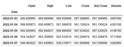
Implementation N°1: Basic
Here are the steps:
- We calculate the 20-day moving average price of Netflix
- We calculate The difference between the price and this moving average
- If the difference is positive, a sell order is triggered. When the difference is negative a buy order is triggered.
On one hand, if the difference is positive, it means that the price is above its moving average 20-day. It means that the asset is overbought and it will revert back (decrease) to this average value. Thus, a sell order is triggered.
On the other hand, if the difference is negative, meaning the asset is oversold, it would tend to increase and reach its average value, hence a buy order is triggered.
Python Code
window = 20
df["ma_20"] = df["Adj Close"].rolling(window=window).mean()
df["diff"] = df["Adj Close"] - df["ma_20"]
df['signal'] = np.where(df["diff"] > 0, -1, 1)
figs=(8,4)
df[['Adj Close',"ma_20"]].plot(figsize=figs)
plt.title("Mean Reversion")
plt.show()
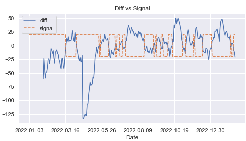
df['diff'].plot(figsize=figs)
#I multiplied the signal by 20 be able to show it clearly in the graph
(20*df['signal']).plot(figsize=figs, linestyle='--')
plt.title("Diff vs Signal")
plt.legend()
plt.show()
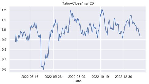
(df["Adj Close"]/df["ma_20"] ).plot(figsize=figs)
plt.title("Ratio=Close/ma_20")
plt.show()I plotted in this graph the price vs its moving average 20 days:

I plotted in this graph the difference (price – its moving average 20days) and also the signal. It shows when buy and sell orders are triggered:
In this graph I plotted the Ratio between the price and its moving average. The goal is to see how the ratio is oscillating. If it’s around one, meaning the price is reverting back to its moving average. We can see clearly that there is a big jump in April 2022.
Limitation
As you can see during the period of April 2022, there was an important decrease in the price of the stock, which continued during several months. If we follow the basic implementation, a buy order would be triggered. Buying at this moment would result in big losses in the following days and months. That’s why one needs to combine this implementation with other indicators, or choose a different calculation method.
Backtesting the strategy
As noticed just before, the sharp drop in price in April 2022 impacts severely the performance of the strategy:
# Backtesting the strategy
# Calculate the daily returns
df['returns'] = df['Adj Close'].pct_change()

# Calculate the strategy returns
df['strategy_returns'] = df['signal'] .shift(1) * df['returns']

# Calculate the cumulative returns
df=df.dropna()
df['cumulative_returns'] = (1 + df['strategy_returns']).cumprod()

figs = (8,4)
# Plot the cumulative returns
df['cumulative_returns'].plot(figsize = figs)
plt.title("Cumulative Return")
plt.show()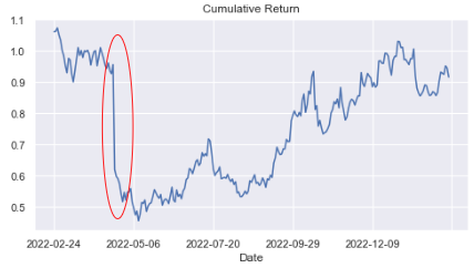
Implementation N°2 : z-score
This implementation can be used in quantitative trading algorithms:
- We calculate the 20-day moving average price
- We calculate the 20-day standard deviation
- We calculate the z-score as:
zscore = (Price- MovingAverage(20days))/StdDev(20days)
If the price crosses the upper band (the moving average 20 days + n_std standard deviation), a sell order is triggered. It means that the instrument is overbought.
If the price goes below the lower band (the moving average 20 days – n_std standard deviation), a buy order is triggered.
Python Code
window=20

# Calculate the 50-day moving average
df['ma_20'] = df['Adj Close'].rolling(window=window).mean()

# Calculate the standard deviation of the 10-day moving average
df['std_20']  = df['Adj Close'].rolling(window=window).std()

# Calculate the z-score (number of standard deviations away from the mean)
df['zscore']  = (df['Adj Close'] - df['ma_20']) / df['std_20']

# Buy order if the z-score is less than n_std (=1)
# Sell order if the z-score is more than n_std (=1)
# Hold if between -1 and 1
n_std=1.25
df['signal'] = np.where(df['zscore'] < -n_std, 1, np.where(df['zscore'] > n_std,-1, 0))

figs=(8,4)
df['signal'].plot(figsize=figs, linestyle="--")
df['zscore'].plot(figsize=figs)
plt.title("Mean Reversion with z-score")
plt.legend()
plt.show()
In this plot, we have the z-score, and also the trading signal for buy or sell orders:

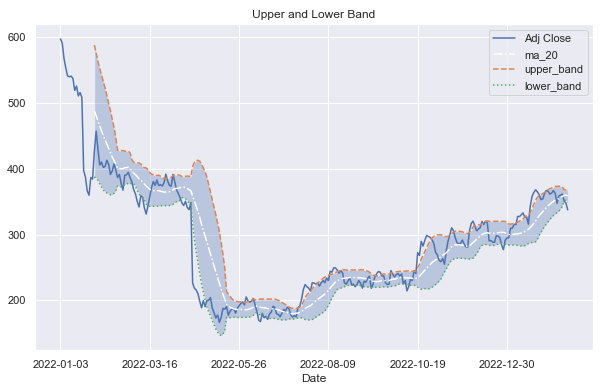
upper_band=df['ma_20']+n_std*df['std_20']
lower_band=df['ma_20']-n_std*df['std_20']

figs=(10,6)
df['Adj Close'].plot(figsize=figs)
df['ma_20'].plot(figsize=figs,linestyle='-.', color="w")
upper_band.plot(linestyle='--',label='upper_band')
lower_band.plot(linestyle=':',label='lower_band')
plt.fill_between(df.index,lower_band, upper_band, alpha=0.3)
plt.title("Upper and Lower Band")
plt.legend()
plt.show()
With this plot, we can see clearly when the price is out of the band. By crossing the upper band, the stock becomes overbought, and this is a signal to enter in a short position.
When the price decreases and crosses out the lower band, the stock becomes oversold, and this can be seen as a buy signal order.
Backtesting the strategy
# Calculate the daily returns
df['returns'] = df['Adj Close'].pct_change()

# Calculate the strategy returns
df['strategy_returns'] = df['signal'] .shift(1) * df['returns']

# Calculate the cumulative returns
df=df.dropna()
df['cumulative_returns'] = (1 + df['strategy_returns']).cumprod()

# Plot the cumulative returns
df['cumulative_returns'].plot(figsize=figs)
plt.title ("Cumulative Return")
plt.show()
This strategy is showing a good performance when n_std=1.25:
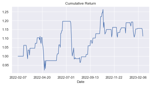
Try to modify this number, to understand the impact it will have on the overall performance.
Comparison
By adding the constraint on how many standard deviations the stock must deviate from its moving average, before triggering the buy or sell order, the performance of this strategy becomes more attractive, compared to the first implementation in the first paragraph.
This implementation can also be used in High-Frequency Trading by adapting the calculation to the intraday prices.
- The intraday prices can be sampled to some seconds, or even milliseconds.
- A rolling mean and standard deviation to be calculated on seconds
- Then a buy or sell order will be triggered if the upper or lower barriers are crossed.
Implementation N°3: Statistical arbitrage
In this implementation, we will be studying the mean reversion of the spread between 2 stocks:
- We calculate the spread in prices between two stocks
- We calculate the moving average 20-day of the spread
- We calculate the moving standard deviation 20-day of the spread.
- We calculate the z-score as:
zscore = (spread – MovingAverage(20days))/StdDev(20days)
Python Code
Loading the dataset of 2 stocks: Apple and Google:
import pandas as pd
import datetime as dt

def download_stock_data(ticker,timestamp_start,timestamp_end):
    url=f"https://query1.finance.yahoo.com/v7/finance/download/{ticker}?period1={timestamp_start}&period2={timestamp_end}&interval
=1d&events=history&includeAdjustedClose=true"
    df = pd.read_csv(url)
    return df

# Determine Start and End dates
datetime_start=dt.datetime(2022, 2, 8, 7, 35, 51)
datetime_end=dt.datetime.today()

# Convert to timestamp:
timestamp_start=int(datetime_start.timestamp())
timestamp_end=int(datetime_end.timestamp())

tickers=['AAPL','GOOG']

df_global=pd.DataFrame()
for ticker in tickers:
    df_temp = download_stock_data(ticker,timestamp_start,timestamp_end)[['Date','Adj Close']]
    df_temp = df_temp.set_index('Date')
    df_temp.columns=[ticker]
    df_global=pd.concat((df_global, df_temp),axis=1)
df_global.head()
Indicators calculation
# Calculate the spread between two stocks:
ticker_long = 'AAPL'
ticker_short = 'GOOG'
spread = df_global[ticker_long] - df_global[ticker_short]

window = 20
n_std = 1.5

# Calculate the rolling mean and standard deviation of the spread
rolling_mean = spread.rolling(window=30).mean()
rolling_std = spread.rolling(window=30).std()

# Calculate the z-score (number of standard deviations away from the rolling mean)
zscore = (spread - rolling_mean) / rolling_std

upper_band = rolling_mean + n_std * rolling_std
lower_band = rolling_mean - n_std * rolling_std
Now we plot the different indicators to see how the spread vs lower and upper band is behaving:
figs=(8,4)
plt.figure(figsize = figs)
spread.plot(label='Spread = '+ticker_long+' - '+ ticker_short,linestyle='--')
df_global[ticker_long].plot(label=ticker_long+'_price')
df_global[ticker_short].plot(label=ticker_short+'_price')
plt.title("Spread and Prices of {0} and {1}".format(ticker_long,ticker_short))
plt.legend()
plt.show()
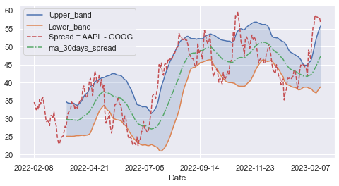
plt.figure(figsize = figs)
upper_band.plot(label='Upper_band')
lower_band .plot(label='Lower_band')
spread.plot(label = 'Spread = '+ticker_long+' - '+ ticker_short,linestyle='--', color='r')
rolling_mean.plot(label = 'ma_30days_spread', linestyle = '-.')
plt.fill_between(df_global.index,lower_band, upper_band, alpha=0.2)
plt.legend()
plt.show()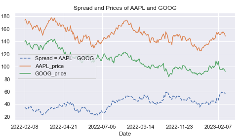
The spread has crossed above or below the upper and lower bands. Thus gives signal trading to buy or short the spread:
Backtesting the strategy
# Enter a long position if the z-score is less than -n_std
# Enter a short position if the z-score is greater than n_std
signal = np.where(zscore < -n_std, 1, np.where(zscore > n_std, -1, 0))
signal = pd.Series(signal, index=df_global.index)

# Calculate the daily returns
returns = df_global[ticker_long].pct_change() - df_global[ticker_short].pct_change()

# Calculate the strategy returns : # Shift the signal by one day to compute the returns
strategy_returns = signal.shift(1) * returns

# Calculate the cumulative returns
cumulative_returns = (1 + strategy_returns).cumprod()

# # Plot the cumulative returns
cumulative_returns.plot(figsize = figs)
plt.title("Cumulative Return with n_std={0}".format(n_std))
plt.show()
The cumulative return produced by this strategy is showing positive value over the whole period.
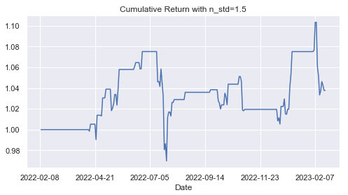
By modifying the number of standard deviations in the model (n_std), you will see the impact on the performance of the strategy. For n_std=1.25, the performance is worse.

Summary
Throughout this article, you have acquired knowledge on the Mean Reversion Trading Strategy Using Python. Additionally, you have explored three distinct approaches for its implementation:
- Basic Implementation: An introductory approach to implementing the algorithm.
- Z-score Indicator Implementation: Utilizing the z-score indicator, commonly applied in quantitative and high-frequency trading.
- Spread of 2 Stocks Implementation: Incorporating the spread of two stocks, a technique commonly employed in statistical arbitrage.
By familiarizing yourself with these implementations, you have gained a comprehensive understanding of the Mean Reversion Trading Algorithm.
I hope you enjoyed reading me.
Leave me a comment to tell me what you think about the content 👇.