Hull Moving Average In Python (HMA)

Algorithmic Trading

This article introduces the Hull Moving Average (HMA) and explores its implementation in Python. You will gain insights into what the HMA is and how it functions, along with two different methods to implement it. Additionally, both strategies will be backtested, and a comprehensive interpretation of the results will be provided.

What is Hull Moving Average (HMA)?

The Hull Moving Average is a type of moving average that is aiming to reduce the lag of a traditional moving average, while still providing a smooth and accurate measure of an asset’s price trend.

The HMA was developed by Alan Hull in 2005 and is calculated using moving averages on different period intervals.

The HMA can be used to identify a trend reversal or to confirm an existing trend.

FORMULA

WMA_1 = Weighted Moving Average (WMA) of the price over period/2
WMA_2 = WMA of the price over period
HMA_non_smooth = 2 * WMA_1 – WMA_2
HMA = WMA of HMA_non_smooth over sqrt(period)

In the following, you will discover how to implement HMA using Python. 2 methods will be detailed and compared to calculate the WMA. A backtesting of these 2 strategies will be also compared.

Hull Moving Average (HMA) Python Implementation

Method 1

Calculate the WMA as a moving average price weighted by the period:

def hma(period):
    wma_1 = df['Adj Close'].rolling(period//2).apply(lambda x: \
                                        np.sum(x * np.arange(1, period//2+1)) / np.sum(np.arange(1, period//2+1)), raw=True)
    wma_2 = df['Adj Close'].rolling(period).apply(lambda x: \
                                        np.sum(x * np.arange(1, period+1)) / np.sum(np.arange(1, period+1)), raw=True)
    diff = 2 * wma_1 - wma_2
    hma = diff.rolling(int(np.sqrt(period))).mean()
    return hma

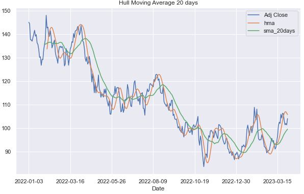
period = 20
df['hma'] = hma(period)
df['sma_20days'] = df['Adj Close'].rolling(period).mean()

figsize = (10,6)
df[['Adj Close','hma','sma_20days']].plot(figsize=figsize)
plt.title('Hull Moving Average {0} days'.format(period))
plt.show()

As shown in the graph, HMA responds more quickly than the usual SMA:

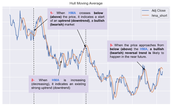
You can try shorter timeframes to see how closely the HMA follows the shape of the price curve.

df['hma_short']=hma(14)
df['hma_long']=hma(30)

figsize = (12,6)
df[['Adj Close','hma_short','hma_long']].plot(figsize=figsize)
plt.title('Hull Moving Average')
plt.show()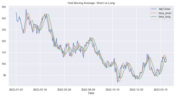

Method 2

Use the volume to calculate the weighted average:

def hma_volume(period):
    wma_1 = df['nominal'].rolling(period//2).sum()/df['Volume'].rolling(period//2).sum()
    wma_2 = df['nominal'].rolling(period).sum()/df['Volume'].rolling(period).sum()
    diff = 2 * wma_1 - wma_2
    hma = diff.rolling(int(np.sqrt(period))).mean()
    return hma

df['nominal'] = df['Adj Close'] * df['Volume']

period = 20
df['hma_volume']=hma_volume(period)

figsize=(12,8)
fig, (ax0,ax1) = plt.subplots(nrows=2, sharex=True, subplot_kw=dict(frameon=True),figsize=figsize)

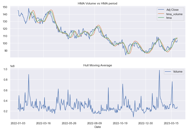
df[['Adj Close','hma_volume','hma']].plot(ax=ax0)
ax0.set_title('HMA Volume vs HMA period')

df[['Volume']].plot(ax=ax1)
ax1.set_title('Hull Moving Average')

plt.show()

The HMA with volume is a bit more lagged than the HMA calculated in the first method:

Backtesting the strategies

To backtest each strategy (method 1 and 2), let’s calculate a short and a long period of HMA:

When the short period crosses above the long period, a buy order can be triggered.

When the short period crosses below the long period, a sell order can be triggered.

Then we calculate the pnl generated by each signal.

Strategy 1

#SIGNALdf['hma_short']=hma(20)
df['hma_long']=hma(30)

df['signal'] = np.where(df['hma_short'] > df['hma_long'],1,-1)

#RETURN
df['signal_shifted']=df['signal'].shift()

## Calculate the returns on the days we trigger a signal
df['returns'] = df['Adj Close'].pct_change()

## Calculate the strategy returns
df['strategy_returns'] = df['signal_shifted'] * df['returns']

# Calculate the cumulative returns
df1=df.dropna()
df1['cumulative_returns'] = (1 + df1['strategy_returns']).cumprod()

#PLOT
figsize=(12,8)
fig, (ax0,ax1) = plt.subplots(nrows=2, sharex=True, subplot_kw=dict(frameon=True),figsize=figsize)

df[['Adj Close','hma_long','hma_short']].plot(ax=ax0)
ax0.set_title("HMA: Short vs Long")
df[['signal']].plot(ax=ax1,style='-.',alpha=0.4)

ax1.legend()
ax1.set_title("HMA - Signals")
plt.show()

df1['cumulative_returns'].plot(figsize=(10,4))
plt.title("Cumulative Return")
plt.show()

You can see then the signals generated at each time there a crossover line:

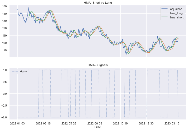
The overall return generated during the whole period of the dataset is positive, even if during some periods it was negative:

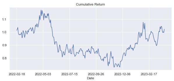
The return:

df1['cumulative_returns'].tail()[-1]

1.0229750801053696

Discover over 25 Technical Indicators, Momentum and Trend Following

With clear, detailed explanations, interpretations, and formulas. hands-on learning with full Python implementation

I’M CURIOUS

Strategy 2

#SIGNAL
df['hma_volume_short']=hma_volume(20)
df['hma_volume_long']=hma_volume(30)
df['signal'] = np.where(df['hma_volume_short'] > df['hma_volume_long'],1,-1)

#RETURN
df['returns'] = df['Adj Close'].pct_change()

# Calculate the strategy returns
df['strategy_returns'] = df['signal'].shift() * df['returns']

# Calculate the cumulative returns
df2=df.dropna()
df2['cumulative_returns_volume'] = (1 + df2['strategy_returns']).cumprod()

#*********************************PLOT*****************************
figsize=(12,8)
fig, (ax0,ax1) = plt.subplots(nrows=2, sharex=True, subplot_kw=dict(frameon=True),figsize=figsize)
df[['Adj Close','hma_volume_short','hma_volume_long']].plot(ax=ax0)
df[['signal']].plot(ax=ax1,style='-.',alpha=0.4)
ax0.set_title("HMA - Volume: Short vs Long")

ax1.legend()
plt.title("HMA - Signals")
plt.show()

figs = (10,4)
df2['cumulative_returns_volume'].plot(figsize = figs)
plt.title("Cumulative Return")
plt.show()

As HMA Volume seems to be more smooth than HMA in the first method, less signals can be triggered (in our example only 1 less):

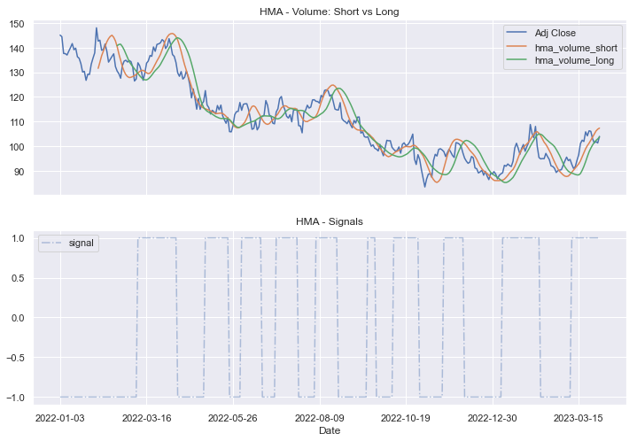
The return generated by this strategy is not that good: 0.75 (0.775-1⇒ -24%)

df2['cumulative_returns_volume'].tail()[-1]

0.7555329108482581

Let’s compare the signal of the 2 strategies:

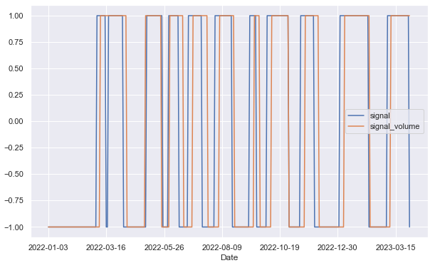
df['signal'] = np.where(df['hma_short'] > df['hma_long'],1,-1)
df['signal_volume'] = np.where(df['hma_volume_short'] > df['hma_volume_long'],1,-1)

figsize=(12,8)
df[['signal','signal_volume']].plot(figsize=figsize)
plt.show()

The signals remain more in the short position than in the long position:

Using the HMA alone can not be enough to generate a profitable strategy. One can use other indicators like the RSI or CCI to detect the zones where the overbought or oversold are happening.

Interpretation

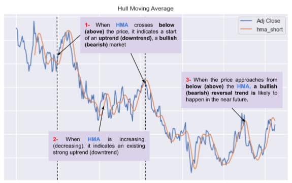
Crossover signals: When the price crosses above the HMA, it can be interpreted as a bullish signal, and when the price crosses below the HMA, it can be interpreted as a bearish signal. It can also trigger buy and sell signals as we already saw before, when comparing slow to fast period HMA (point 1-).

Trend-following signals: The HMA can also be used to identify trends and generate trend-following signals. When the HMA is sloping upwards, it indicates an uptrend, and when it’s sloping downwards, it indicates a downtrend (point 2-).

Reversal signals: When the price is approaching the HMA from below, a bullish reversal trend can happen in the near future.